Secant’s calculations answer three practical questions:
Where is the signal strongest? Compare activations from two prompt groups, then test the resulting direction on held-out examples. Signal-to-noise ratio (SNR) measures separation relative to variation within the groups.
How can several edits coexist? Make their output directions perpendicular before combining them. This removes linear overlap between the chosen vectors, not all interaction between model behaviors.
How large should the edit be? Use the layer’s reference activation to calculate a requested output shift. A weight change of the same relative size can have different effects in different layers or models.
A writer is a matrix that contributes to a layer’s output. The residual stream is the running activation vector passed between transformer layers. A norm measures a vector’s length or a matrix’s size; the Frobenius norm is the square root of the sum of squared matrix entries. Below, D holds protected directions as rows. The labels B1, B2, and B3 refer to loop, refusal, and root-cause directions in the reported experiments.
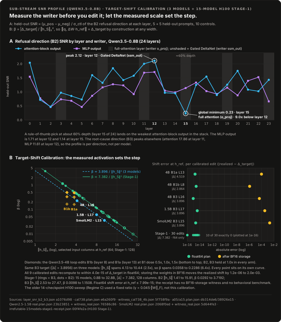
Figure 1:A. Held-out SNR of the B2 refusal direction on Qwen3.5-0.8B, by layer and writer. This panel uses the margin statistic from the layer sweep (5 + 5 held-out prompts, 10 controls), not the of Section 1, so its values are not comparable to the H100 numbers. Layer 15, where a rule of thumb at about 60% depth lands, is the global minimum of the attention-block output (0.23) and is a full-attention layer (writer o_proj); layer 12, a Gated DeltaNet layer (writer ssm_out), peaks at 2.12.
B. Every calibrated rank-1 edit in the banked plans: the B3 target is the same on Qwen3.5-4B, Qwen2.5-1.5B and SmolLM2-1.7B, spans 4.13 to 10.44, and spans 0.0358 to 0.2286. Recomputing from each plan in float64 gives ; after the weights are stored in BF16 the realized shift moves by to . Generated from the banked receipts by gen_secant_figures.py, which checks every receipt’s SHA-256 before drawing.
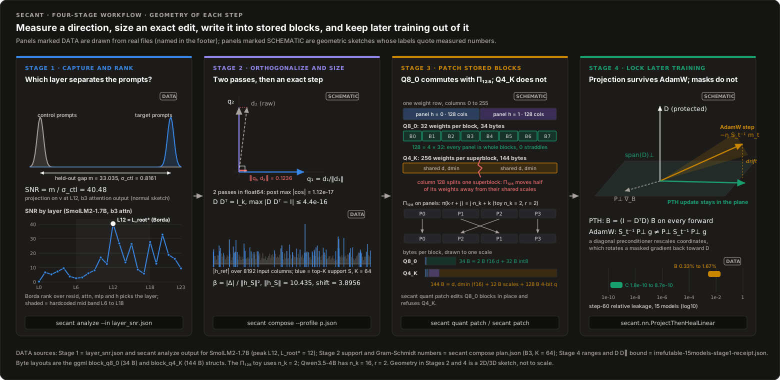
Figure 2:Sections 1 to 4 of this page explain Stages 1 and 2. Stage 1 shows what an SNR measures: the target prompts’ projections onto a direction sit m = 33.0 away from the control prompts’, with control spread σ = 0.816, so SNR = 40.48 at L12 of SmolLM2-1.7B. Below that is the per-layer curve that secant analyze ranks. Stage 2 shows Section 3’s two Gram-Schmidt passes, which take a raw cosine of 0.1236 to 1.12e-17, and Section 2’s sparse support. The B3 edit uses only the 64 of 8,192 input columns where is largest, so fixes for the requested shift 3.8956. Stages 3 and 4 are covered in quantized surgery and Project-Then-Heal.
1. Compare Two Prompt Groups on Held-Out Data
Capture records the activations for each group. One half of the data chooses a candidate direction; the other tests it. Swapping the halves gives a second check. This reduces reuse of the fitting data, but choosing among many layers still needs a separate final evaluation set.
Let denote the activation exiting layer (either in the residual stream or a specific writer sub-stream such as attn_out / ssm_out or mlp_out) at the final prompt token of input . Capture collects a positive class and a negative class . The two classes are not paired and need not have equal size; every statistic below is computed from separate class means and separate class variances, in float64 (python/secant/capture.py, evaluate_cell).
Splits. Each class is shuffled independently with a fixed seed derived from (seed, stream) and cut into half (the first samples) and half (the rest). For a sample set , write for the class means and
for the unit difference-of-means direction fitted on . The reported direction is fitted on all samples.
Unbiased variances. For a scalar sample , (ddof=1). For a vector class on split , , the sum of the unbiased per-coordinate variances.
Two Signal-to-Noise Measures Answer Different Questions
In high-dimensional residual streams (), the trace denominator sums within-class variation across all coordinates, keeping raw trace SNR modest (0.32 to 4.88 across the 12 full H100 models, with microsoft/phi-4 an outlier at up to 909.6) even when a 1D concept direction cleanly separates the two prompt classes. The projected statistic instead measures variance along one fitted direction only. Secant evaluates three diagnostics, each fitted on one half and scored on the other:
Projected (1D) Signal-to-Noise Ratio (
snr_proj). Fit on half and score the projections on half :The same is computed with the roles swapped (), and the reported value is the average over the two splits:
Both directional values are also recorded (
snr_proj_a_to_b,snr_proj_b_to_a).Trace (full-space) Signal-to-Noise Ratio (
snr_trace). This uses no fitted direction; “fit on ” only selects which half is scored:With finite samples the numerator also contains noise, so under independent isotropic class noise with variance , the numerator’s noise contribution is . This is not a bias formula for the SNR ratio itself; neither statistic is null-corrected.
Split-Half Cosine Stability (
split_half_cosine). The cosine between the directions fitted independently on each half:Near
1means the two fitted directions agree; near0means they do not. Independent isotropic random directions have cosine approximately , but a small cosine alone does not prove the data contain no signal.
The 1D projected SNR and the trace SNR answer different questions: asks how well one held-out direction separates the classes, while compares the mean shift with the total variance of the whole space. They are not interchangeable and are never divided into one another.
Undefined cells. If a mean difference vanishes (relative to , below 10-12) or a denominator is zero or non-finite, the cell is reported as status="undetermined" with NaN metrics and a reason, never as a number. Capture requires at least 4 samples per class so each half has a variance.
The reported experimental selection heuristic treats a candidate layer as admissible if and . These thresholds are permissive: every peak layer used for an edit in the H100 runs is far above them, so in practice the highest score selects the layer. These are not enforced CLI acceptance gates. Selecting a maximum over layers on these splits requires a separate evaluation set before making an unbiased generalization claim.
2. Edit a Small Set of Input Columns
The MLP is the transformer’s feed-forward block. Its down-projection maps a wider internal activation back into the residual stream. A sparse edit changes selected input columns. A rank-1 edit is the outer product of one output direction and one input selector, scaled by an edit strength.
Let be the MLP down-projection matrix at layer , which maps intermediate SwiGLU activations into the residual stream:
Rather than modifying all columns of , Secant selects the top- intermediate neurons (, typically ) with the largest absolute reference activations in the Rust composer, and constructs a column-sparse selector vector supported solely on . Here is the reference activation used to select those columns:
With unit-length output direction and normalized selector , a rank-1 column-sparse update with step size takes the form:
Because (e.g., of columns on Qwen3.5-4B), over 99% of the logical matrix entries lie outside the edit. In a quantized file, re-encoding a touched block can also change reconstructed values of other entries in that block.
3. Remove Overlap Between Edit Directions
Gram-Schmidt subtracts components that earlier directions already cover, then normalizes the remainder. The result depends on the direction order. Two passes reduce numerical error; directions that cannot supply an independent component are rejected.
When behavioral edits share the coordinate basis , non-orthogonal directions can interfere constructively or destructively.
Given , secant compose applies two-pass modified Gram-Schmidt orthogonalization in float64 to produce a normalized row basis . Rust and Python enforce the full Gram-matrix contract (python/secant/_linalg.py, ORTHONORMALITY_TOL):
Both implementations reject a residual norm below 10-9 of the input norm, non-finite inputs/intermediates, and full Gram error at or above 1e-12. Norms use overflow-resistant fallback/scaling for finite rescalings. The measured float64 residual on tested bases is below 10-15: the maximum over 120 seeded Gaussian bases (, , , 5 seeds each) was .
The multi-subspace update is then synthesized over the orthogonalized directions :
4. Match an Edit to a Reference Activation
Calibration asks for a particular change at one measured input to the writer. It divides that target by the energy in the selected input columns. The equality below holds in exact arithmetic at that reference input; rounding and other inputs require separate checks. A fixed weight-norm ratio sizes an edit by the weights instead, so the two choices need not produce the same activation shift.
Suppose we want a writer matrix update to induce a target inner-product shift along unit direction when presented with reference input activation , where denotes zeroed outside the selected column support and satisfies the non-degeneracy precondition :
Then the induced output shift along at is exact by construction:
and the Frobenius norm of the update adapts automatically to the layer’s activation scale:
When reference activation norms are not pre-captured, secant compose also supports a relative Frobenius perturbation mode scaled by a dose multiplier :
The modes size different quantities: the calibrated step depends on the measured activation , the ratio step only on . The signed in this derivation is the target after the profile’s sign and value rules have been applied. Rust takes its magnitude from the selected calibration value and its sign from slot.sign; a nonzero slot target precedes the flag, followed by the profile default. projector-subtract uses its own gamma path.
Target-shift composition preserves the combined rank1 contribution along the original unit directions. Write their columns as with upper-triangular . For a common reference activation and support, solve , equivalently . With different reference activations or selected columns, the triangular entry also includes the sparse coefficient row evaluated on the requesting activation. Distinct tensor pairs are independent systems. Projector edits remain separate, base-dependent transformations; their weight changes are not included in the additive target-shift promise. Inconsistent GGUF/SafeTensors tensor bindings are rejected in target-shift mode. The NumPy helper cross_projection_compensate implements the common-reference system. For and with targets , the combined update is , giving both requested projections. Gamma mode continues to dose the orthogonalized basis.
Relation to prior associative-memory and abliteration estimators. Algebraically, is the isotropic (, minimum-Frobenius-norm Moore-Penrose pseudoinverse) special case of the rank-1 ROME update (Meng et al., NeurIPS 2022; extended to multi-edit MEMIT, ICLR 2023) restricted to sparse top- column support , while whitened concept erasure was formalized in LEACE (Belrose et al., NeurIPS 2023). Multi-vector Gram-Schmidt orthogonalization and ridge-regularized projection appear in G-Abliteration (Gülmez, Dec 2025), Norm-Preserving Biprojected Abliteration (Lai, Nov 2025), Obliteratus, llm-abliteration, apostate KCRN, and weightless. Secant’s specific contributions here are using activation-calibrated target shifts ( and RMS-relative dosing ) for cross-model-size edit transfer (0.8B to 32.8B across 15 full models, plus 70.6B and 72.7B single-shard evaluations) and solving the upper-triangular cross-projection compensation system () for heterogeneous non-orthogonal directional edits.
Reported experiments. Full Target-Shift Calibration () was used on Qwen3.5-4B (all B1+B2+B3 edits; <think> closure 0/30 in a05, where only B1 was at and B2 and B3 were held at , then 21/30 with all three at and 30/30 in a15, where B1 was at and B2 and B3 again at ) and on the B3 edit of SmolLM2-1.7B and of Qwen2.5-1.5B (see the calibration figure, panel B). The 14-checkpoint H100 sweep (7.2B to 72.7B) used the fixed-ratio mode (); there, aligned directions separate from equal-norm random directions by 29.1x to 1,269.9x by magnitude. A random unit direction projects onto with expected magnitude about , so this is a geometric sanity check, not evidence of behavioural change.
The 15-model H100 Stage-1 run (0.8B to 32.8B, receipt irrefutable-15models-stage1-receipt.json, SHA-256 00f4fe2afc4ff630c7c9ac55b5b2c0a85342477a5b32a0b0c455abd5b4c5056f) applied full Target-Shift Calibration to B2 and B3 on every model, with and 128 selected input columns. Across B2, spans 1.41 to 15.91 and spans 0.0292 to 3.7192; across B3, 2.53 to 27.47 and 0.0098 to 1.1508. Every one of the 30 edits realizes its target at with maximum error approximately 7.99e-15 in float64 (10 of them exactly 0). Each random control is norm-matched. This run has no BF16-storage witness and its behavioral benchmarks are NOT_RUN, so it establishes that the step is solved correctly at every width tested, not what the edit does to generated output.
B2 / B3: refusal / root-cause directions; L: layer; support norm: L2 norm of the selected reference activations; β: calibrated step size.
Max error: largest float64 reference-shift error over B2 and B3; it is repeated to keep each direction readable on its own.
B2 calibration
| Model (size) | B2 layer | Support norm | B2 β | Max error |
|---|---|---|---|---|
| Qwen3.5-0.8B (0.8B) | L17 | 3.57 | 0.5801 | 8.9e-16 |
| SmolLM2-1.7B (1.7B) | L17 | 14.14 | 0.0369 | 1.8e-15 |
| Qwen3.5-4B (4B) | L23 | 12.35 | 0.0484 | 3.6e-15 |
| Mistral-7B-v0.3 (7.2B) | L12 | 2.81 | 0.9352 | 3.6e-15 |
| Qwen2.5-7B (7.6B) | L8 | 7.77 | 0.1224 | 2.7e-15 |
| Llama-3.1-8B (8B) | L23 | 4.03 | 0.4556 | 1.8e-15 |
| R1-Llama-8B (8B) | L23 | 4.12 | 0.4343 | 5.3e-15 |
| Qwen3-8B (8.2B) | L14 | 4.33 | 0.3931 | 5.3e-15 |
| Gemma-2-9B (9.2B) | L16 | 1.41 | 3.7192 | 1.8e-15 |
| OLMo-2-13B (13.7B) | L16 | 8.08 | 0.1130 | 3.6e-15 |
| Phi-4 (14.7B) | L12 | 2.54 | 1.1436 | 4.4e-15 |
| Qwen3-14B (14.8B) | L16 | 4.97 | 0.2994 | 1.8e-15 |
| R1-Qwen-14B (14.8B) | L28 | 14.66 | 0.0343 | 3.6e-15 |
| Gemma-2-27B (27.2B) | L14 | 9.35 | 0.0845 | 8.0e-15 |
| Qwen3-32B (32.8B) | L47 | 15.91 | 0.0292 | 3.6e-15 |
B3 calibration
| Model (size) | B3 layer | Support norm | B3 β | Max error |
|---|---|---|---|---|
| Qwen3.5-0.8B (0.8B) | L14 | 4.53 | 0.3595 | 8.9e-16 |
| SmolLM2-1.7B (1.7B) | L12 | 5.20 | 0.2727 | 1.8e-15 |
| Qwen3.5-4B (4B) | L16 | 4.40 | 0.3805 | 3.6e-15 |
| Mistral-7B-v0.3 (7.2B) | L19 | 12.03 | 0.0510 | 3.6e-15 |
| Qwen2.5-7B (7.6B) | L14 | 7.05 | 0.1484 | 2.7e-15 |
| Llama-3.1-8B (8B) | L16 | 3.82 | 0.5070 | 1.8e-15 |
| R1-Llama-8B (8B) | L16 | 3.96 | 0.4701 | 5.3e-15 |
| Qwen3-8B (8.2B) | L21 | 9.82 | 0.0766 | 5.3e-15 |
| Gemma-2-9B (9.2B) | L25 | 2.53 | 1.1508 | 1.8e-15 |
| OLMo-2-13B (13.7B) | L20 | 15.06 | 0.0325 | 3.6e-15 |
| Phi-4 (14.7B) | L29 | 20.61 | 0.0174 | 4.4e-15 |
| Qwen3-14B (14.8B) | L23 | 11.62 | 0.0547 | 1.8e-15 |
| R1-Qwen-14B (14.8B) | L35 | 20.44 | 0.0177 | 3.6e-15 |
| Gemma-2-27B (27.2B) | L27 | 27.47 | 0.0098 | 8.0e-15 |
| Qwen3-32B (32.8B) | L25 | 10.00 | 0.0738 | 3.6e-15 |
What the same edits do to generated output. A later public-benchmark receipt (public-benchmarks/irrefutable-receipt.json, SHA-256 9859ef3e...3132) ran these exact aligned edits on 14 of the 15 models (Gemma-2-27B is HOLD). Each model answered GSM8K, MATH-500, MMLU-Pro, HumanEval, and 30 crash traces at 1.0x and 1.5x. A control set ran with norm-matched random directions: the same and support , with replaced by a random unit vector orthogonal to it. The control is what makes the result readable. A correct reference shift does not by itself say what an edit costs, and comparing against an equal-size random edit separates the effect of direction from the effect of magnitude.
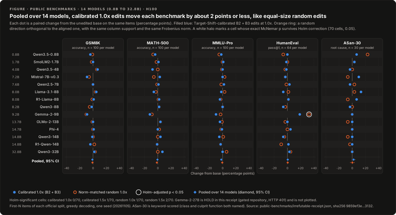
Figure 3:Paired change from base for each model and benchmark, calibrated 1.0x (blue) against norm-matched random 1.0x (orange). No calibrated cell survives Holm correction (0/70). Pooled over 14 models, calibrated edits move each benchmark by -2.0 to +2.1 points, and random edits by -1.4 to +0.4. The one model that moves a lot, Gemma-2-9B, has the sweep’s largest step, from , and its random control moves as far as its calibrated edit. A small makes large, so check it before trusting a reference shift as a dose. Method and tables: paper, Section 4.2.
Size the Target Relative to the Writer’s Output (RMS-Relative Dosing)
A target such as or 1.0 is an absolute number. Whether it is large depends on how large the writer’s outputs already are. RMS-relative dosing measures that first, over positive reference activations , and then asks for a fraction of it:
The step is solved exactly as above, so the reference-input identity still holds. Only the size of the request changes. Across our 6-model RMS-calibrated sweep (Qwen2.5-Math-7B-Instruct, Qwen2.5-Coder-7B-Instruct, DeepSeek-R1-Distill-Llama-8B, Qwen3-4B, Qwen3-8B, and Qwen3-14B, totaling 24,000 benchmark evaluations), spans 5.847 (DeepSeek-R1-Distill-Llama-8B layer 21) to 78.148 (Qwen3-8B layer 24). On layer 19 of Qwen2.5-Math-7B-Instruct, over 24 references, so an earlier run that asked for a unit shift of 1.0 was at (1.34% of the output norm), too small to change greedy answers (GSM8K 87, MATH-500 43 of 100, with no complete cell moving more than 1 point). Across all 6 models at , the unhealed four-domain composed edit matched its norm-matched random control. Adding ProjectThenHealLinear (composed_healed_rms_1p0x, 3.18e-17 to 5.07e-17 relative subspace leakage) raised GSM8K from 87 to 93 on Qwen2.5-Math-7B-Instruct (unadjusted p = 0.031), HumanEval from 36 to 42 on Qwen2.5-Coder-7B-Instruct (unadjusted p = 0.238), and HumanEval from 5 to 12 on DeepSeek-R1-Distill-Llama-8B (unadjusted p = 0.092), though none survives Holm correction across the full test family; direct 60-step heal-the-base (base_lora_1p0x) and healed-random (random_healed_rms_1p0x) control arms show that on Qwen2.5-Math-7B-Instruct both controls also reach 93 on GSM8K (p = 1.000, attributing the 87 -> 93 gain to the LoRA pass itself while ProjectThenHealLinear cuts domain-subspace leakage from 4.75% to 5.08e-17), whereas on Qwen2.5-Coder-7B-Instruct HumanEval base_lora_1p0x (37) and random_healed_rms_1p0x (35) do not reproduce composed_healed_rms_1p0x (42, p = 0.332 and 0.189).
On the paired ASAN-120 vulnerability and patched-benign twin benchmark (9 models 7 arms, 7,560 evaluations; paper, Section 4.5), pairing 60 vulnerable C/C++ snippets with 60 patched benign twins shows that all 5 non-reasoning models (0.8B to 8B) collapse to trivial one-sided predictors (BA = 0.475 to 0.533, RC <= 0.067), whereas on the 4 <think> reasoning models (R1-Distill-Llama-8B, Qwen3-8B, Qwen3-14B, Qwen3-32B), composed_rms_1p0x beats random_rms_1p0x 4/4 on balanced accuracy (6W / 1L / 2T across all 9 models, exact sign-test p = 0.125, mean dBA = +0.017) and lifts strict root-cause recall (RC = verdict + class + sink) from 0.183 to 0.250 (+6.7 pp over base, +11.7 pp over random_rms_1p0x) on R1-Distill-Llama-8B and from 0.450 to 0.550 (+10.0 pp over base, +8.3 pp over random_rms_1p0x) on Qwen3-14B. Two practical rules follow. Report next to any absolute target, so readers can tell a negligible dose from a large one. And treat calibration as exact only at the reference inputs: on benchmark prompts the same edits moved the writer output by 0.5% to 14.8% of its norm, depending on direction. Full tables: paper, Sections 4.4 and 4.5.